
What is Varve Chronology?
Varve chronology is the use of varve sequences to establish time lines in sedimentary sequences and for correlation. The advantage that varves have over other sediments is that they have tremendous precision of a year and in some cases down to the level of seasonal layers within a varve if intra-annual stratigraphy shows a consistent separation of seasonal features. Correlation of glacial varve records from place to place is generally based on the matching of the pattern of varve thickness change and not absolute thickness, which varies widely for a single varve year across a lake or region. In addition, correlations can sometimes be established by matching basin-wide lithologic changes in varve sequences if they represent isochronous events.
Some Preliminary Terminology
Throughout this web site the terms varve record, varve series, and varve chronology are used to denote varve sequences of different hierarchical status. The term “varve sequence” is used as a generic term to refer to any succession of varves regardless of whether they are single outcrop records or represent larger, more regional correlations involving many varve records.
Varve record: A measured string of varves from a single exposure or drill core. The annual numbering of a record is temporary and will change as errors are eliminated when it is matched to a series or chronology and it is corrected to the numbering system of the higher order sequence.
Varve series: A number of varve records that have been matched from a relatively constrained area and together make a longer and more accurate sequence than a single varve record. Numbering of a series often starts at 1 at the bottom (oldest varve) and implies a higher level of accuracy than can be achieved with a single varve record.
Varve chronology: A correlation of varve series and records that together have a uniform numbering system and apply to a broader region than a varve sequence, perhaps from different lakes or valleys. A varve chronology will grow as it incorporates series and smaller chronologies over time. Because of regional annual correlations of varve sequences a varve chronology is implied to have a greater accuracy and more regional applications for correlation.
In glacial environments varve sequences are used to establish time lines for such things as deglaciation or the repopulation of regions by organisms following deglaciation. Varve sequences allow us to fix very precisely in varve years the age of any fossil or sediment feature found in the varves or the varve age of any event that may be tied to the varve sequence. Sediment features found in varve sequences include abnormally thick sandy beds marking flood events and volcanic ash beds. In Sweden, deglaciation as well as the history of marine incursion and isostatic uplift in the Baltic Sea basin have been relatively dated using varve sequences where late Pleistocene and Holocene glacial lake and brackish water marine deposits are varved and represent long periods of time.
Varve sequences and records represent floating time scales or time scales that are not fixed according to their true or calendar ages. To use a varve sequence to establish the true or calendar ages of events it is necessary to calibrate the sequence with numerical ages. The technique which has been used most frequently to do this in glacial varve sequences is radiocarbon (14C) dating. In Sweden, varve sequences may be calibrated by simply counting varves because the youngest varves are historic and come up to the present. The count of varves back from the present then gives an estimate of the absolute age of the sediment provided that the varve sequence does not have any gaps or the lengths of gaps can be estimated precisely.
To construct a varve record in glacial lacustrine sediment the thicknesses of annual layers are counted and measured to formulate a time scale of varve years and corresponding varve thickness. The block of sediment shown here is from the deposits of Lake Vermont, a late Pleistocene glacial lake that occupied the Champlain Valley of New York.
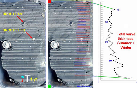
Dried block of varved clay, Boquet R., Willsboro, NY
These varves were deposited in a position very distal to the receding glacier and also are from the relatively shallow flanks of Lake Vermont where less sediment was deposited during the summer than in deeper parts of the basin. As a result, winter layers are thicker here than summer layers. Still, summer layers vary more in thickness than winter layers. The thicknesses of summer and winter layers are recorded as shown with the posted red and blue lines. Red lines represent the bottoms of summer layers and blue lines mark the bottoms of winter layers. Total annual layer (summer + winter) thickness for 36 varves is plotted on the graph to the right. A data file and the lines posted on the image were all created by a computer program designed to sequentially measure varve sequences. The pattern shown on the plot, or varve record, should be distinctive of the time during which the varves were deposited. Annual layer thickness varies as weather patterns that control meltwater and sediment input to the lake vary from year to year. Long term thickness changes reflect changing patterns of sedimentation resulting from such things as changes in sediment sources and distribution patterns, climate change, and vegetation patterns on the land adjacent to the lake.
Using Varve Records for Correlation and as Time Scales
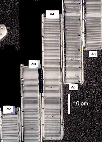
Dried cores A2-A6, Newbury, VT, site no. 73 of Antevs (1922)
Matching Varve Cores: Annual Thickness Variation and Intra-annual Stratigraphy
To assemble a glacial varve record at an outcrop, overlapping cores can be matched or spliced according to thickness patterns and intra-annual features seen in specific varves. Shown here are matching varve cores from the lower part of a varve section at Newbury, VT in the Connecticut Valley. Drying of the cores may lead to a slight reduction in varve thickness but the pattern of change from year to year is still preserved.
Matching Outcrop Records
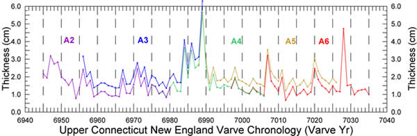
Varve records from matched cores at a single exposure can be averaged to produce a composite record. Shown below are the overlapping cores in the Newbury section shown at right. Cores A2-A6 collected at Newbury, Vermont (Antevs’ site no. 73) in 1996 are matched to each other. Cores A3 and A5 have been shifted upward 0.5 cm to prevent coincident lines from being concealed on the plot. Averaged values of these matching cores, which are nearly identical, were used to assemble an outcrop record.
Matching an Outcrop Record to an Existing Chronology
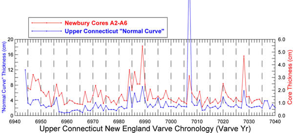
Next, the compiled varve record (averaged values) from overlapping cores A2-A6 at Newbury, VT (Antevs’ site no. 73) are matched to the New England Varve Chronology’s upper Connecticut “normal curve” of Antevs (1922). The two records are plotted against axes with different scales on opposite sides of the graph. They have very similar thicknesses, with the outcrop record being slightly thinner, except for a large spike in the “normal curve” at varve 7007 that is not recorded as strongly at the Newbury section. Antevs’ compilation was done further up the Connecticut Valley than Newbury and closer to the source of the sediment that produced the spike. The spike is represented by a sandy bed just above the top of core A4 in cores A5-6 on the varve core image and likely represents the release of water from a lake dammed in a tributary of the Connecticut Valley north of Newbury.
Matching Outcrop Varve Records with Normal Curves
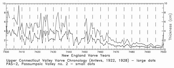
Below, is the composite varve record from cores 25-33 (upper line) at PAS2 (Passumpsic Valley, East Barnet, VT) that has been averaged and matched to the upper Connecticut normal curve of the New England Varve Chronology (lower line) of Antevs (1922, 1928). Both records are plotted at the same scale with varves at PAS2 being thicker. Note that in some places, for example at 7403 and 7439-7449 the PAS2 exposure had sediment deformation and varves could not be measured. The rest of the sequence matched the New England Varve Chronology showing precisely how many years were missing from the PAS2 exposure. The matching of varve records for correlation here is based on changes in the thickness pattern of varves and not absolute thickness, which varies widely for a single varve year in a lake or across a region. The PAS2 section could not have been used to compile new varve stratigraphy without matching it to other sections to fill gaps in the PAS2 record.
The sediment block from the Champlain Valley and the Newbury cores used above as examples were measured using digital images and a computer measurement program. The original varve records assembled in Sweden and in New England a century ago were measured at the outcrop and recorded on a tape pinned to a vertical face. This technique still works well but is not as accurate when varves are clayey or thin, making them difficult to distinguish in the field. Collecting overlapping core samples and digital images also guarantees that measurements can be reviewed later and cores can be sampled for analysis of other features in the varves such as fossils or sediment types. For more information on measuring varves, see the Field Varve Measurement page.